Reply to Comments Made by R. Grave De Peralta Menendez and
S.L. Gozalez Andino
Appendix II
Introduction
This Appendix extends the results presented in [1]. Here, regularized instantaneous, 3D,
discrete, linear solutions for the EEG inverse problem are considered.
Here I make two propositions. First, ordinary cross-validation is the method of choice
for selecting the regularization parameter. Second, in a comparative study of inverse solutions,
the method of choice is the inverse solution with minimum cross-validation error. All this work
is based on the contributions of Stone [12].
There are two methodological principles involved in judging the performance of an inverse solution:
1. An inverse solution is "not good" if it has high cross-validation error.
2. The converse is not true.
Very informally, the principle states that the selected model must produce the best prediction
(in the true sense of objective prediction, as in e.g., the leave-one-out procedure). It is
important to emphasize the "prediction error" as defined in the work of Stone [12]
is a concept very different from the classical one used in "goodness of fit"
and in "least squares".
1. Methods
The reader must refer to [1] for background and notation.
The regularized version of the generalized minimum norm inverse problem considered is:
| |
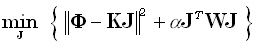 |
(20) |
for any given positive definite matrix W of dimension (3M) • (3M),
and for any given α > 0.
This problem and its solution can be found
in [6], equations (9), (9'), (10), (10') therein.
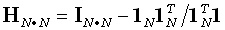
Note that K and Φ belong to the
linear manifold  (HN), where HN
is the N • N
average reference operator (or centering
matrix) defined as:
(HN), where HN
is the N • N
average reference operator (or centering
matrix) defined as:
| |
 |
(21) |
where 1N is an N•1
vector composed of ones. In this case, rank (K) = (N - 1),
K ≡ HN K,
and Φ ≡ HN Φ.
The solution to the problem in equation (20) is:
| |
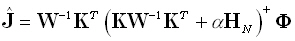 |
(22) |
The cross-validation error is defined as:
| |
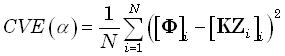 |
(23) |
where [Φ]i denotes the
ith element of Φ,
[KZi]i
denotes the ith
element of the vector KZi,
and:
| |
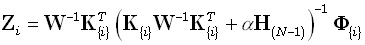 |
(24) |
where K{i} is obtained from K by
deleting its ith row;
K{i}∈(H(N-1));
K{i} ≡ H(N-1) K{i};
Φ{i} is obtained from Φ
by deleting its ith
element; and Φ{i} ≡ H(N-1) Φ{i}.
An equivalent equation for cross-validation error is:
| |
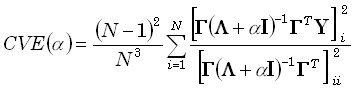 |
(25) |
where KW-1KT = ΓΛΓT denotes the eigen-decomposition;
Γ is an N•(N-1)
matrix whose columns are eigenvectors;
and Λ is an (N-1)•(N-1)
diagonal matrix with non-null eigenvalues.
Three important comments:
1. These equations are valid if the matrix W does not depend on the measurement space,
i.e., it must not depend on the position or number of electrodes.
2. Equation (25) is valid for any α ≥ 0.
3. I have emphasized here the use of simple ordinary cross-validation as the
"common yard stick" for comparing inverse solutions. Ordinary cross-validation
corresponds exactly to the concept of "prediction error" based on "leave one
out". Furthermore, it can be calculated exactly for any inverse solution (linear,
non-linear, Bayesian, etc.). Generalized cross-validation does not have these properties.
______________________________